반응형
이번에는 sklearn을 사용하지 않고 logistic regression을 모델링하고 차근차근 gradient descent, cost, weight등을 학습 할때마다의 변화를 그래프로 표현까지 해보는 예제를 포스팅 해보겠습니다. 역시나 logistic regression의 개념은 여러 위키 블로그, 서적등에 매우 잘 설명 되어있으므로 생략하겠습니다.
데이터 읽어와서 plot 그리기
import pandas as pd
import matplotlib.pyplot as plt
import numpy as np


df = pd.read_csv('logistic_regression_data.csv') # csv 파일 읽기


x= df.iloc[:, 1: -1].values # 입력값
y= df.iloc[: , -1].values #클래스

plt.scatter(x[:, 0][y == 0], x[:, 1][y == 0], marker='o',color='red', label='0') # 플랏 뿌려주기
plt.scatter(x[:, 0][y == 1], x[:, 1][y == 1], marker='x',color='blue', label='1')
plt.legend(["class 0", "class 1"], loc=4)
plt.grid(True)
plt.xlabel("x")
plt.ylabel("y")

plt.title("1")
plt.show()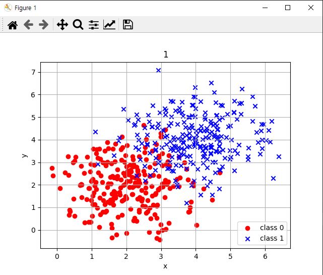
데이터를 읽어와서 plt.scatter로 입력데이터 2개를 라벨 0,1로 나누어 그린 그래프입니다. 2차원 평면으로 표시했고 maker와 color등은 보기편하시게 고르시면 됩니다.
logistic regression 구성
sigmoid
def sigmoid(z):
    return 1 / (1 + np.exp(-z))
gradient descent
def grad(w, X, Y):
    y_pred = hx(w,X)
    g = [0]*3
    g[0] = -1 * sum(Y*(1-y_pred) - (1-Y)*y_pred)
    g[1] = -1 * sum(Y*(1-y_pred)*X[:,0] - (1-Y)*y_pred*X[:,0])
    g[2] = -1 * sum(Y*(1-y_pred)*X[:,1] - (1-Y)*y_pred*X[:,1])
    return g


def descent(w_new, w_prev, lr,iter ,w_plot=False,c_plot=False):
    #print(w_prev)
    w_new_R = []
    cost_R = []
    for i in range(0,iter):
        w_prev = w_new
        w0 = w_prev[0] - lr * grad(w_prev, x, y)[0]
        w1 = w_prev[1] - lr * grad(w_prev, x, y)[1]
        w2 = w_prev[2] - lr * grad(w_prev, x, y)[2]
        w_new = [w0, w1, w2]
        cost_R.append(cost(w_new, x, y))
        w_new_R.append(w_new)
        #print(w_new)
cost
def cost(w, X, Y):
    y_pred = hx(w,X)
    return -1 * sum(Y*np.log(y_pred) + (1-Y)*np.log(1-y_pred))
epoch에 따른 cost, weight 변화 그래프 표시
cost 그래프
epoch에 따른 손실률을 나타내는 그래프입니다. 점차 줄어들며 마지막에는 더이상 내려가지 않는 모습을 보입니다. 학습이 잘되고 있다는걸 눈으로 확인할 수 있습니다.
def plot_cost(alpha, epoch):

    w = [1, 1, 1]

    cost = descent(w, w, alpha, epoch,w_plot=False,c_plot=True)

    iter_num = range(len(cost))

    plt.scatter(iter_num, cost, label='cost')

    plt.xlabel("Iterations"); plt.ylabel("cost")
    plt.legend()

    plt.title("HW2")
    plt.show()


epoch = 100
alpha_lst = 0.001 #학습 rate

plot_cost(alpha_lst,epoch)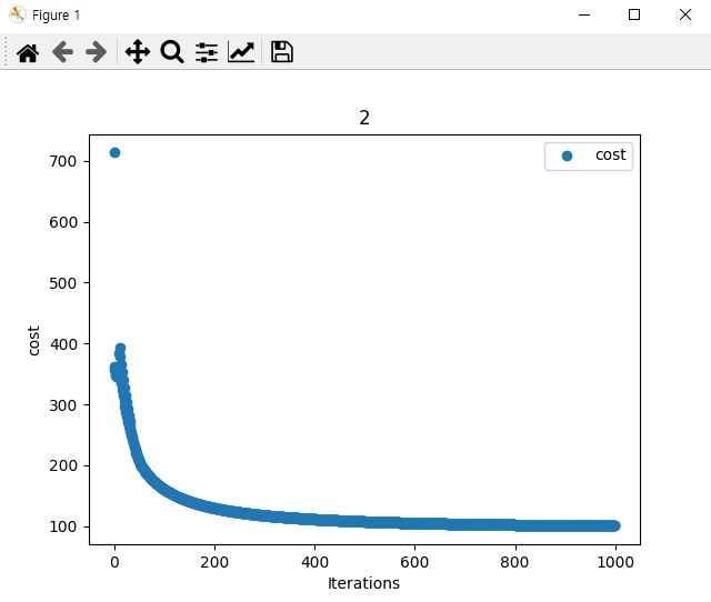
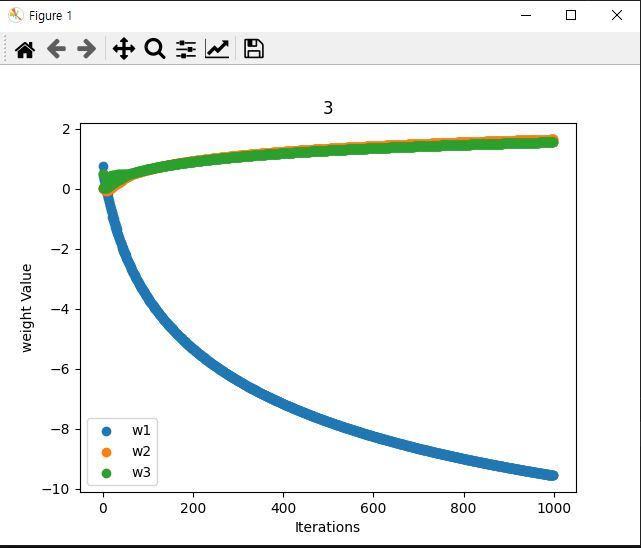
weight 그래프
epoch당 가중치의 변화값을 표현하는 그래프입니다. 모든 학습과정을 완료 한뒤 최적의 매개변수 가중치를 가지고 정확도를 판단합니다.
def plot_weight(alpha, epoch):

    w = [1, 1, 1]

    w = descent(w, w, alpha, epoch,w_plot=True,c_plot=False)

    iter_num = range(len(w))
    new_weight1= []
    new_weight2 = []
    new_weight3 = []
    for i in range(0,len(w)):
        new_weight1.append(w[i][0])
        new_weight2.append(w[i][1])
        new_weight3.append(w[i][2])

    plt.scatter(iter_num, new_weight1, label='w1')
    plt.scatter(iter_num, new_weight2, label='w2')
    plt.scatter(iter_num, new_weight3, label='w3')


    plt.xlabel("Iterations"); plt.ylabel("weight Value")
    plt.legend()

    plt.title("HW3")
    plt.show()

epoch = 100
alpha_lst = 0.001 #학습 rate
plot_weight(alpha_lst,epoch)
logistic regression 결정 경계선 그래프 그리기
학습된 가중치를 가지고 마지막으로 logistic regression 결정 경계선을 그릴 차례입니다. 입력데이터가 2개 출력은 1개이므로 가중치는 총 3개 w0,w1,w2가 되겠습니다.
def graph(form, x_range):
    x = np.array(x_range)
    y = form(x)

    plt.plot(x, y)


def get_form(x):
    return (-result_w[0] - result_w[1] * x) / result_w[2]

graph(get_form, range(0,7))

plt.scatter(x[:, 0][y == 0], x[:, 1][y == 0], marker='o',color='red', label='0')
plt.scatter(x[:, 0][y == 1], x[:, 1][y == 1], marker='x',color='blue', label='1')

plt.legend(["", "class 0","class 1"], loc=4)
plt.grid(True)

plt.xlabel("x")
plt.ylabel("y")

plt.title("5")
plt.show()
모델 정확도 계산
def accuracy_score(y_true, y_pred):
    count = 0
    y_pred = y_pred>0.5
    for true, pred in zip(y_true, y_pred):
        if true == pred:
            count += 1
    return count/len(y_true)*100

y_pred=hx(result_w,x)


print("정확도 : "  +str(accuracy_score(y,y_pred)) + '%' )
이상으로 sklearn 없이 logistic regression을 구현하고 여러 그래프를 그리며 배운 이론대로 잘 그려지는지 확인 용도로 logistic regression 예제코드로 사용하시면 될것 같습니다.
반응형
'개발' 카테고리의 다른 글
| Keras Conv2d CNN 간단한 예제 ( Mnist data) (0) | 2022.05.24 |
|---|---|
| 파이썬 opencv 이미지 색상 추출 히스토그램 RGB 그래프 그리기 예제(colorHistogram, color 그래프 ) (0) | 2022.05.23 |
| (ETL) TALEND OPEN STUDIO DB 데이터 엑셀로 출력하기(MSSQL) (0) | 2022.05.18 |
| sklearn 사이킷런 SVM모델 그래프 그리기 (margin, decision boundary) (0) | 2022.05.16 |
| (ETL) TALEND OPEN STUDIO를 설치해보자. (0) | 2022.05.12 |


댓글